
Part 1: Introduction & Getting Started with Excel
What is Microsoft Excel?
Microsoft Excel is a powerful spreadsheet software developed by Microsoft, designed for organizing, analyzing, and visualizing data. It’s part of the Microsoft Office suite and has become a standard tool across industries—used by professionals, students, and businesses alike.
From simple data tracking to complex financial modeling, Excel offers an intuitive interface for both beginners and experts.
Why Learn Excel?
Whether you’re managing household expenses, running a small business, or analyzing scientific data, Excel is a universal tool with wide-ranging benefits:
- Data organization: Use spreadsheets to store and retrieve data logically.
- Automation: Automate repetitive tasks with formulas and macros.
- Career boost: Proficiency in Excel is a top skill in many job descriptions.
- Decision-making: Visualizations and summaries help in better business decisions.
- Versatility: Excel is used in finance, HR, marketing, education, and tech sectors.
💡 Explore how Excel complements technical skill development.
How to Install and Open Excel
There are several ways to access Excel depending on your system and preferences:
- Microsoft 365 Subscription: This is the most popular method, offering Excel on desktop and online, with cloud sync and regular updates.
- Standalone Excel: You can purchase Excel as a one-time license through Office Home & Student or Office Professional packages.
- Excel Online: A free, browser-based version accessible via a Microsoft account at Office.com.
Understanding the Excel Interface
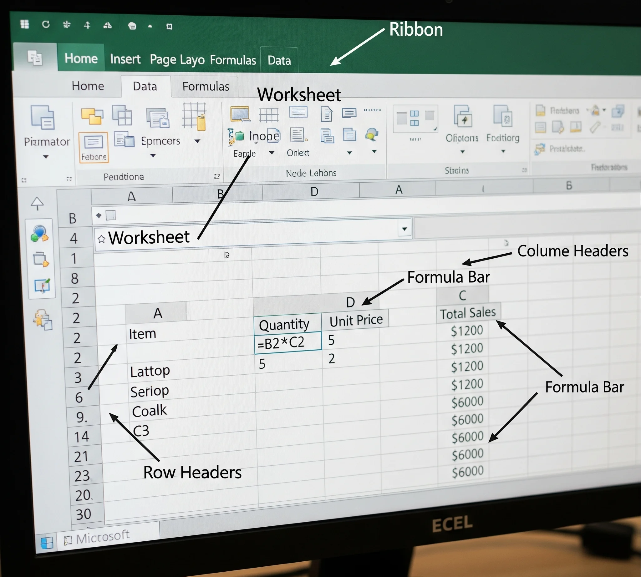
Before jumping into data entry or formulas, let’s understand the Excel interface elements:
- Ribbon: The toolbar at the top with tabs like Home, Insert, Formulas, Data, and View.
- Worksheet Area: The grid where your data lives—organized into rows and columns.
- Formula Bar: Shows the content of the selected cell, especially useful for formulas.
- Quick Access Toolbar: Lets you customize shortcuts like Save, Undo, and Redo.
- Status Bar: Displays info like average, count, and sum of selected cells.
Creating and Saving a Workbook
To get started:
- Open Excel and select Blank Workbook.
- Enter your data or create a template.
- Click File > Save As and choose a format:
.xlsx— Default Excel format.xls— Legacy format for older versions.csv— Plain text, comma-separated format for data exchange
Excel Navigation Basics
Getting comfortable with navigation helps you work faster:
- Use the Arrow Keys to move cell-by-cell.
- Use Ctrl + Arrow Key to jump to the edges of data regions.
- Ctrl + Page Up/Page Down to switch between worksheets.
- Use the Name Box to go to a specific cell or named range.
💡 Tip: Press Ctrl + Home to return to cell A1 instantly.
Part 2: Core Excel Functions and Formulas
What is a Formula in Excel?
In Excel, a formula is an expression that calculates the value of a cell. Every formula begins with an = sign, followed by the expression to compute. For example:
=A1 + B1Formulas can include functions, operators, cell references, and constants.
Commonly Used Functions
Functions are pre-built formulas that perform specific calculations. Here are some essential ones:
=SUM(A1:A5)– Adds values in a range.=AVERAGE(B1:B10)– Calculates the mean.=MIN(C1:C10)– Returns the smallest number.=MAX(D1:D10)– Returns the largest number.=COUNT(E1:E20)– Counts numerical entries.=COUNTA(F1:F20)– Counts all non-empty cells.=ROUND(G1, 2)– Rounds to two decimal places.
Logical Functions
Logical functions evaluate conditions and return results based on TRUE or FALSE outcomes:
=IF(A1>100, "High", "Low")– Returns “High” if A1 is greater than 100.=AND(A1>0, B1<10)– Returns TRUE only if both conditions are met.=OR(A1>100, B1<5)– Returns TRUE if either condition is met.=NOT(A1=0)– Returns TRUE if A1 is not equal to 0.
Lookup & Reference Functions
These functions help search for and return data from different cells or ranges:
=VLOOKUP(lookup_value, table_array, col_index, FALSE)– Searches vertically.=HLOOKUP(lookup_value, table_array, row_index, FALSE)– Searches horizontally.=XLOOKUP(lookup_value, lookup_array, return_array)– Newer, flexible replacement for VLOOKUP.=INDEX(array, row_num, [column_num])– Returns the value at a specific position.=MATCH(lookup_value, lookup_array, match_type)– Returns the position of a value.
💡 Tip: Combine INDEX and MATCH for dynamic lookups across large datasets.
Text Functions
These functions help manipulate and clean text-based data:
=LEFT(text, num_chars)– Extracts characters from the beginning.=RIGHT(text, num_chars)– Extracts characters from the end.=MID(text, start_num, num_chars)– Extracts a substring from the middle.=TRIM(text)– Removes extra spaces from text.=TEXT(value, format_text)– Formats numbers as text (e.g. date formatting).=CONCAT(text1, text2,...)– Joins multiple pieces of text together.
Date & Time Functions
Use these to work with dates and time values:
=TODAY()– Returns the current date.=NOW()– Returns current date and time.=DATEDIF(start_date, end_date, "Y")– Calculates years between dates.=EOMONTH(start_date, months)– Returns the last day of the month after a given number of months.
Want to Learn More Formulas?
🧠 Explore Excel Jet’s extensive formula library for quick, practical examples of every Excel function.
Part 3: Formatting, Data Management, and Visualization
Cell Formatting Basics
Proper formatting improves readability and clarity in Excel. Here are basic formatting features you can apply from the Home tab:
- Font styles: Bold, Italic, Underline
- Font color and fill color: Highlight key data
- Cell borders: Define sections in your data table
- Number formatting: Change between currency, date, percentage, etc.
💡 Tip: Use the Format Painter to quickly copy formatting from one cell to another.
Conditional Formatting
Conditional formatting visually emphasizes important data based on rules:
- Highlight Cell Rules: Values greater than, less than, or equal to a number
- Data Bars: Shows relative size as a bar inside the cell
- Color Scales: Gradient colors based on value ranges
- Icon Sets: Traffic lights, arrows, and symbols to classify data
To apply, go to Home > Conditional Formatting and choose a rule.
Data Validation & Drop-down Lists
Control data input and avoid errors using Data Validation:
- Select a range of cells
- Go to Data > Data Validation
- Choose List as the validation criteria
- Enter values (comma-separated) or reference a range
This is useful for creating dropdown menus for categories like departments, countries, or product names.
Sorting and Filtering Data
Excel lets you easily sort and filter data to find what matters most:
- Sort by column: A to Z or Z to A (text), smallest to largest (numbers)
- Custom Sort: Sort by multiple levels (e.g., Region, then Sales)
- Filter: Show or hide data based on selected criteria
Access these features under the Data tab. Click the funnel icon to apply filters.
Working with Tables
Convert ranges into tables for better structure and functionality:
- Select your data range
- Click Insert > Table
- Ensure “My table has headers” is checked
Benefits of using Excel Tables:
- Automatic formatting
- Structured references in formulas
- Auto-expansion when adding rows or columns
Charts and Graphs
Data visualization is a key part of Excel’s power. Popular chart types include:
- Column and Bar Charts: Compare values across categories
- Line Charts: Track trends over time
- Pie Charts: Show proportions of a whole
- Combo Charts: Combine two chart types for dual-axis analysis
To insert a chart:
- Select your data
- Go to Insert > Charts
- Choose the chart type that fits your data best
You can also customize chart elements like titles, legends, data labels, and axes under Chart Tools.
Working with Pivot Tables
A Pivot Table is an advanced tool to summarize large datasets with just a few clicks:
- Click anywhere inside your dataset
- Go to Insert > PivotTable
- Choose where to place the table (new or existing worksheet)
From there, drag and drop fields into:
- Rows – Categories
- Columns – Subcategories or time periods
- Values – Metrics (e.g., sum of sales)
- Filters – To filter the entire PivotTable
PivotTables make it easy to slice and dice your data without altering the original dataset.
More Excel Visualization Ideas?
💡 Explore advanced visual dashboards by learning how to create dynamic top 10 lists in Excel with conditional formatting, XLOOKUP, and Pivot Tables.
📌 Learn how visualization tools like Excel can enhance team productivity and decision-making.
Part 4: Advanced Excel Techniques
Named Ranges
A named range is a human-readable label assigned to a cell or range. It makes formulas easier to read and manage.
To create one:
- Select the cell or range.
- Go to Formulas > Define Name.
- Assign a name like
Sales2025.
Now you can use =SUM(Sales2025) instead of a cell range.
Dynamic Ranges with OFFSET and INDIRECT
Use the OFFSET and INDIRECT functions to reference dynamic ranges that adjust as your data grows.
=OFFSET(A1, 0, 0, COUNTA(A:A), 1) creates a range that expands as rows are added.
Dynamic ranges are especially useful for dropdown lists and charts.
Introduction to Macros and VBA
Macros are recorded actions that automate tasks. For more advanced automation, you can use VBA (Visual Basic for Applications).
To record a macro:
- Go to View > Macros > Record Macro.
- Perform your actions in Excel.
- Stop recording. You can now replay the macro.
For example, use VBA to auto-format reports or apply rules to large datasets. VBA code begins with Sub MacroName() and ends with End Sub.
Data Analysis Tools
Excel offers built-in tools for solving data problems:
- Goal Seek: Reverse-engineers the input needed to reach a target result.
- Solver: Optimizes a solution by changing multiple variables under constraints.
- Scenario Manager: Compares multiple “what-if” scenarios.
Find these tools under Data > What-If Analysis.
Power Query Basics
Power Query is a tool for importing, cleaning, and transforming data. No coding required!
- Go to Data > Get & Transform Data.
- Choose your data source (Excel, CSV, Web, SQL, etc.).
- Edit, remove columns, split text, and format dates visually.
Power Pivot and Data Modeling
Power Pivot allows you to build relationships between multiple tables and write advanced DAX (Data Analysis Expressions) formulas.
This is especially useful for complex dashboards or large datasets imported from external sources.
To enable Power Pivot, go to File > Options > Add-ins and enable the Power Pivot add-in.
Collaboration and Sharing
Excel Online and Microsoft 365 support real-time collaboration:
- Comments: Right-click any cell and click New Comment.
- Share workbook: Use File > Share or the Share button on the ribbon.
- Version history: View and restore previous versions under File > Info.
💡 Tip: Protect your worksheet under Review > Protect Sheet to lock editing permissions.
Troubleshooting Formulas
Common formula errors in Excel:</p>
#DIV/0!– Division by zero#VALUE!– Wrong data type used in formula#NAME?– Misspelled function name or range#REF!– Invalid cell reference (e.g., deleted cell)
Use Formulas > Error Checking or Trace Precedents/Dependents to debug issues.
🔗 Related Resource
🧠 Microsoft Excel Official Support has detailed tutorials for each advanced feature.
📌 Read how Excel skills enhance technical leadership in project environments.
Part 5: FAQs, Tips & Resources
Frequently Asked Questions
These are real questions people search for on Google related to learning Excel. Here are clear, concise answers:
What are the basics of using Excel?</h5>
Start by understanding the Excel interface — worksheets, cells, columns, and rows. Learn to enter and format data, apply simple formulas like =SUM(), and explore chart creation and sorting/filtering data.
How do I learn Excel step by step?
Begin with data entry, formatting, and basic functions. Then move on to logical formulas, lookups (VLOOKUP/XLOOKUP), and data visualization. Finally, explore advanced topics like PivotTables, Power Query, and Macros.</p>
What is Excel used for?
Excel is used for data analysis, financial modeling, project tracking, budgeting, scheduling, CRM, inventory tracking, and more. It’s highly versatile and used in nearly every industry.
<h5>Can I teach myself Excel?</h5>
Yes! With online tutorials, YouTube videos, and free resources, you can become proficient in Excel on your own. Practice regularly and work on real-life projects to reinforce skills.
What is the difference between Excel formulas and functions?
Formulas are custom expressions you create, while functions are predefined formulas built into Excel (like =SUM(), =AVERAGE()</code>).
How to use Excel for accounting?
Create templates for invoices, track expenses using categories, apply SUMIF functions for subtotals, and use PivotTables for summary reports. Excel is widely used in bookkeeping and finance.
How to use Excel for project management?
Use Excel to create Gantt charts, assign tasks, track progress, manage deadlines, and allocate resources. Templates and conditional formatting can make project dashboards easy to read.
💡 and planning.
Top Excel Tips for Beginners
- Freeze Panes: Keep headers visible while scrolling – View > Freeze Panes
- Flash Fill: Auto-completes values based on patterns – use Ctrl + E
- AutoFill: Drag formulas or patterns across cells quickly
- Keyboard Shortcuts: Use Ctrl + Arrow Keys to navigate fast
- Use Templates: Start with pre-made templates for budgets, invoices, etc.
Free Resources to Learn More
- – Official tutorials from Microsoft
- ExcelJet – Practical formulas and shortcuts for all levels
- – Ask questions and learn from real-world use cases
Conclusion and Next Steps
Learning Excel is a long-term investment in your personal and professional growth. Start simple, apply what you learn, and explore progressively complex functions and tools. As you gain experience, you’ll unlock new capabilities that help you become more efficient and data-driven.
Your article helped me a lot, is there any more related content? Thanks!