
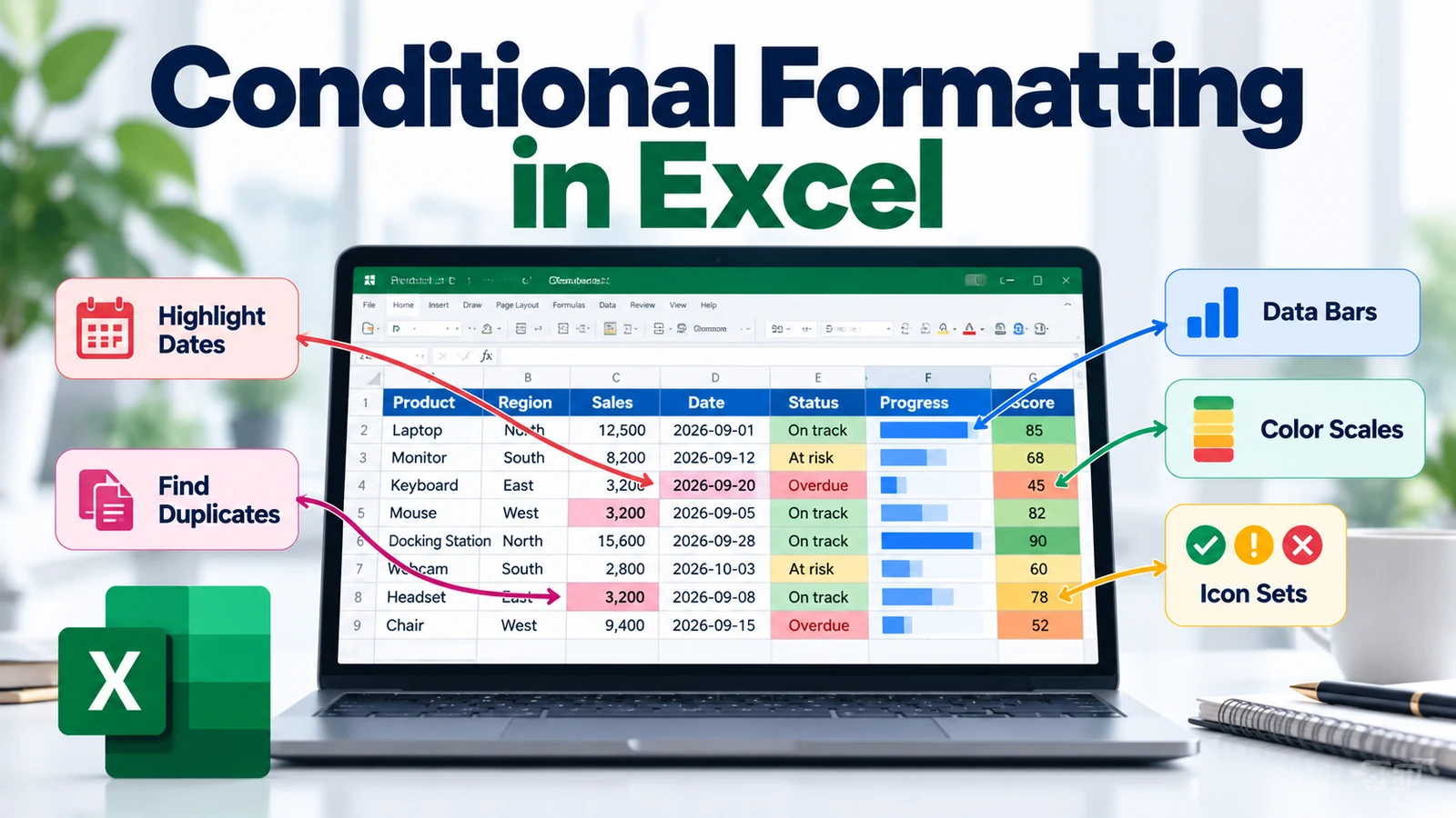
Conditional formatting in Excel helps you make important values, exceptions, patterns, and trends stand out automatically. Instead of reviewing every row manually, you can apply rules that change a cell’s appearance when specific conditions are met.
This practical guide explains how to use conditional formatting in Excel for thresholds, duplicates, dates, percentages, data bars, color scales, icon sets, and formula-based rules. It also shows how project managers can use conditional formatting to highlight overdue tasks, budget variances, risks, and status changes.
If you are building your Excel skills step by step, start with the Microsoft Excel Learning Hub. For calculations behind more advanced rules, use our Excel Formulas and Functions guide. If you are summarizing large datasets, see our PivotTable step-by-step guide.
Microsoft’s official documentation explains how to use conditional formatting to highlight information, how to apply data bars, color scales, and icon sets, and how to apply conditional formatting with formulas for more customized visual rules.
What Is Conditional Formatting in Excel?
Conditional formatting applies a visual format when a rule evaluates as true. The underlying value in the cell does not normally change; only its appearance changes.
For example, you can make Excel automatically:
- Highlight overdue dates.
- Flag duplicate values.
- Mark high-risk items.
- Show values above or below a threshold.
- Apply color scales to performance data.
- Add data bars to compare magnitudes.
- Display icon sets for status or trends.
- Highlight entire rows based on one cell.
Microsoft notes that conditional formatting can be applied to ranges, Excel Tables, and—on supported versions—PivotTable reports. The available options can vary slightly between Windows, Mac, and Excel for the web.
Why Use Conditional Formatting?
Conditional formatting is useful because it converts raw values into visual signals.
Instead of reading every number in a long table, you can immediately spot:
- Exceptions
- Outliers
- High and low values
- Deadlines
- Performance trends
- Duplicates
- Threshold breaches
That can make reports easier to review and reduce the risk of overlooking an important value.
How to Apply Conditional Formatting in Excel
The basic workflow is simple:
- Select the cells you want to format.
- Go to Home > Conditional Formatting.
- Choose a rule type.
- Define the condition.
- Choose the visual format.
- Confirm the rule.
Microsoft also provides Quick Analysis in supported versions of Excel, which can offer conditional-formatting options based on the selected data.
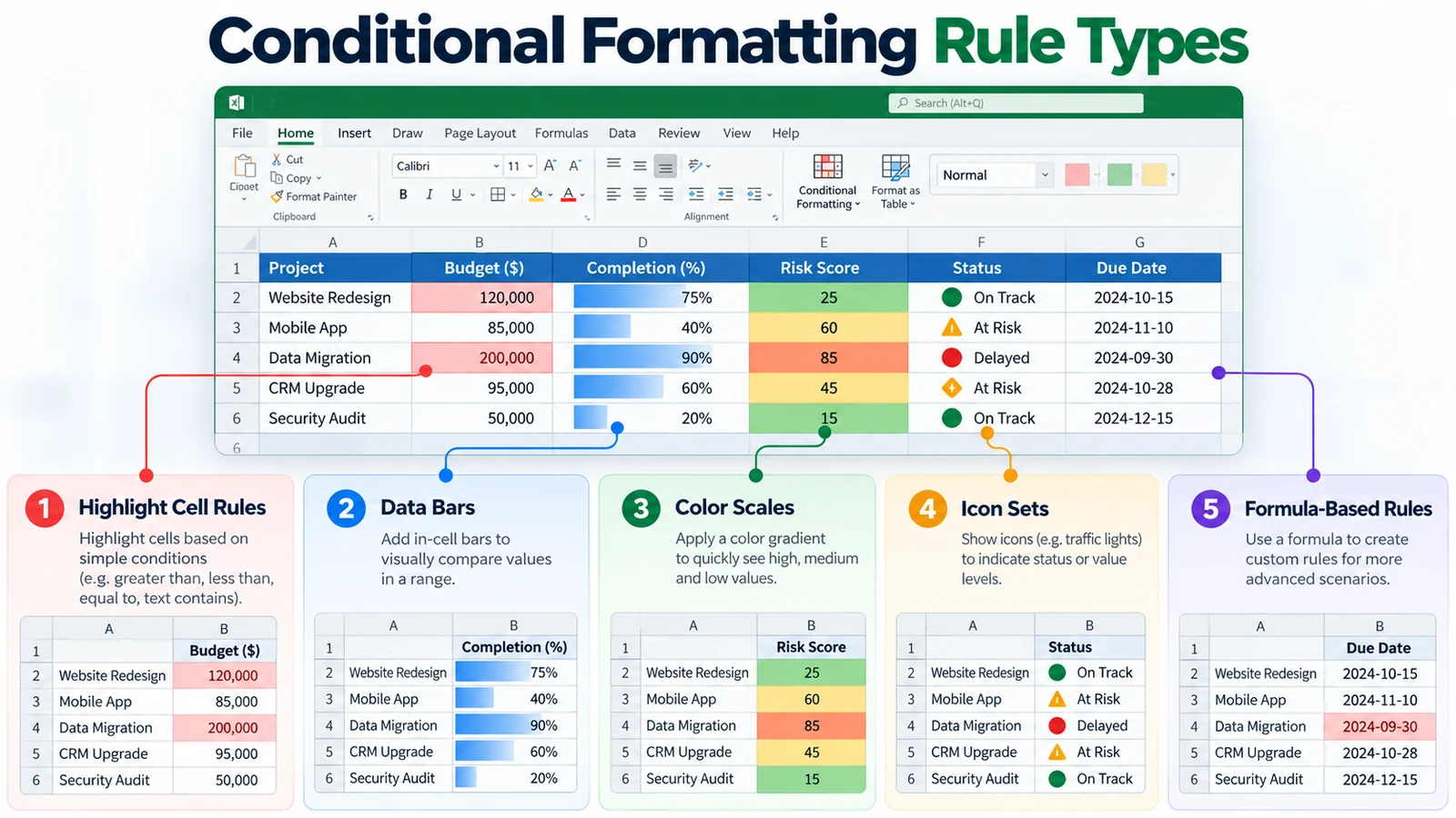
Highlight Cell Rules
Highlight Cell Rules are useful for simple comparisons.
Common rule types include:
- Greater Than
- Less Than
- Between
- Equal To
- Text That Contains
- A Date Occurring
- Duplicate Values
Example: Highlight Values Above a Target
Suppose column C contains monthly revenue and the target is 100,000.
You can select the range and create a rule for:
Cell Value > 100000Excel can then automatically highlight all values above the threshold.
Top and Bottom Rules
Top/Bottom Rules help identify relative performance inside a dataset.
Examples include:
- Top 10 Items
- Top 10%
- Bottom 10 Items
- Bottom 10%
- Above Average
- Below Average
These rules are useful when the threshold should depend on the distribution of the selected data instead of a fixed number.
Use Data Bars to Compare Values
Data bars add a horizontal bar inside each cell. Microsoft explains that longer bars represent larger values and shorter bars represent smaller values, making comparisons easier across a range.
Typical use cases include:
- Sales by region
- Budget usage
- Task completion percentages
- Resource allocation
- Performance scores
To apply them:
Home > Conditional Formatting > Data BarsThen choose a gradient or solid style.
Use Color Scales to Show Distribution
Color scales use two or three colors to represent lower, middle, and higher values. Microsoft describes them as a way to understand distribution and variation in a range.
They work well for:
- Heat maps
- Sales performance
- Risk scoring
- Cycle times
- Survey results
- Utilization percentages
Use them carefully. Too many colors can make a worksheet harder to interpret, especially when the meaning of the scale is not obvious.
Use Icon Sets for Status and Thresholds
Icon sets classify values into categories using symbols such as arrows, circles, flags, or indicators. Microsoft notes that icon sets can divide values into three to five threshold-based categories.
They can be useful for:
- Red / amber / green project status
- Trend direction
- Performance bands
- Priority indicators
- Threshold monitoring
For example, an icon rule could show:
- Green for values at or above 90%
- Amber for values between 70% and 89%
- Red for values below 70%
How to Highlight Duplicate Values
Duplicates are common in imported data, lists, and manually maintained trackers.
To highlight them:
- Select the relevant range.
- Go to Home > Conditional Formatting > Highlight Cell Rules > Duplicate Values.
- Choose the format.
This highlights possible duplicates without deleting anything.
If you later want to remove duplicates, use our complete guide to removing duplicates in Excel.
How to Highlight Dates
Date-based rules are useful for deadlines, renewals, milestones, and follow-up actions.
Common examples include:
- Dates before today
- Dates occurring this week
- Dates occurring next month
- Deadlines within seven days
Example: Highlight Overdue Tasks
If column D contains due dates and column E contains task status, a formula-based rule can highlight only tasks that are overdue and not complete.
=AND($D2<TODAY(),$E2<>"Done")This formula returns TRUE when the due date has passed and the status is not Done.
Conditional Formatting with Formulas
Built-in rules cover many scenarios, but formula-based rules give you more control. Microsoft explains that formula-based conditional formatting must return TRUE or FALSE for the formatting to apply.
To create one:
- Select the target range.
- Go to Home > Conditional Formatting > New Rule.
- Choose Use a formula to determine which cells to format.
- Enter the formula.
- Choose the format.
- Confirm the rule.
Example: Highlight an Entire Row
Suppose column C contains project status and your table starts in row 2.
=$C2="At Risk"If the rule is applied across the whole table range, the entire row can be highlighted whenever the status in column C is At Risk.
Example: Highlight Budget Overruns
If column D is Planned Cost and column E is Actual Cost:
=$E2>$D2This identifies rows where actual spending exceeds the plan.
Example: Highlight High-Priority Open Items
=AND($B2="High",$C2="Open")This is useful in action trackers, issue logs, or risk registers.
Relative vs Absolute References in Conditional Formatting
Formula-based rules are sensitive to cell references.
For example:
=C2="Open"uses a relative reference that can move as Excel evaluates different cells.
=$C2="Open"locks the column but allows the row to change.
This distinction is especially important when you want to highlight an entire row based on one field.
For a deeper explanation, see our Excel Formulas and Functions guide.
How to Manage Conditional Formatting Rules
As a worksheet grows, you may accumulate several rules.
Use:
Home > Conditional Formatting > Manage RulesFrom the Rules Manager, you can:
- Review existing rules
- Edit thresholds
- Change the Apply To range
- Reorder rules
- Delete rules
- Duplicate rules
Microsoft’s Rules Manager also allows you to control the scope of rules in a worksheet.
Rule Order and Stop If True
When several conditional formatting rules apply to the same cells, rule order can matter.
Excel evaluates rules according to the order shown in the Rules Manager. In some scenarios, Stop If True can prevent lower-priority rules from being evaluated after a higher-priority rule succeeds.
This is important when you create multiple status colors or overlapping business rules.
How to Clear Conditional Formatting
To remove formatting rules from selected cells:
Home > Conditional Formatting > Clear RulesYou can clear rules from:
- Selected cells
- The entire worksheet
Microsoft also documents rule deletion through the Conditional Formatting Rules Manager.
Conditional Formatting in Excel Tables
Conditional formatting works well with Excel Tables because Tables provide a consistent structure for growing datasets.
For example, you can apply a rule to a Status column and keep the workbook visually consistent as new rows are added.
Tables also work well as source data for PivotTables. If your next step is summary analysis, continue with our How to Create a PivotTable in Excel guide.
Conditional Formatting in PivotTables
Microsoft notes that conditional formatting can also be used with PivotTable reports, although there are extra considerations for fields in the Values area.
This can be useful when you want to emphasize:
- High-performing categories
- Low-performing regions
- Above-average values
- Top or bottom results
If the PivotTable layout changes, review how the formatting rule is scoped so the visual result remains correct.
Conditional Formatting for Project Managers
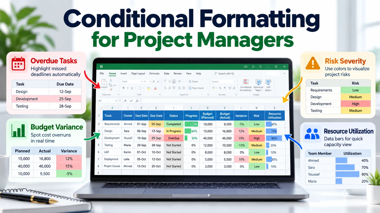
Project managers can use conditional formatting to turn trackers and reports into visual control tools.
1. Overdue Tasks
Highlight tasks whose due date is before today and whose status is not complete.
2. Budget Variance
Highlight projects where Actual Cost exceeds Planned Cost.
3. Risk Severity
Use color scales or icons to distinguish Low, Medium, High, and Critical risks.
4. Action Status
Use different visual signals for Open, In Progress, Blocked, and Complete actions.
5. Schedule Health
Highlight milestones due within the next seven days or milestones already overdue.
6. Resource Utilization
Use data bars or color scales to compare workload percentages across teams.
Common Conditional Formatting Mistakes
Using Too Many Colors
When every cell is highlighted, nothing stands out. Keep the visual language simple.
Using Formatting Without a Clear Meaning
A color should communicate something specific. If red means “overdue,” do not reuse red for an unrelated category in the same report.
Applying Rules to the Wrong Range
Always verify the Apply To range in the Rules Manager.
Incorrect Relative and Absolute References
A formula can work correctly in one row but fail across the full range if references are not designed properly.
Overlapping Rules
Multiple rules can compete for the same cells. Check rule order when the visual result is unexpected.
Ignoring Formula Errors
Microsoft notes that conditional formatting may not be applied when a formula returns an error. Test the underlying formulas and use error-handling logic when appropriate.
Conditional Formatting Best Practices
- Use formatting to support a decision, not just decoration.
- Keep color meanings consistent.
- Limit the number of competing rules.
- Use formulas when built-in rules are not specific enough.
- Test relative and absolute references carefully.
- Review the Apply To range after adding rows or changing layouts.
- Use Tables for structured, growing datasets.
- Keep a simple visual hierarchy for dashboards and management reports.
Conditional Formatting vs Data Validation
| Need | Conditional Formatting | Data Validation |
|---|---|---|
| Highlight important values | Excellent | Not its main purpose |
| Restrict user input | No | Excellent |
| Create visual status signals | Excellent | Limited |
| Create drop-down lists | No | Yes |
These two features work well together. Data Validation controls what users can enter, while conditional formatting changes the visual appearance based on the resulting value.
See our Excel Drop-Down List guide for the Data Validation side of this workflow.
Frequently Asked Questions
Does conditional formatting change the cell value?
No. It normally changes how a value is displayed, not the underlying value itself.
Can conditional formatting use formulas?
Yes. Formula-based rules can evaluate more complex conditions and can reference other cells in the same workbook.
Can I highlight an entire row?
Yes. Apply the rule to the full row range and use a formula that locks the relevant column, such as =$C2="At Risk".
Can conditional formatting work with dates?
Yes. You can use built-in date rules or formulas involving functions such as TODAY().
Can conditional formatting work in PivotTables?
Yes, with some extra considerations around scope and Value fields. Microsoft documents specific behavior for PivotTable reports.
How do I find all conditional formatting rules?
Open Home > Conditional Formatting > Manage Rules and review the scope shown in the Rules Manager.
Continue Learning
Final Takeaway
Conditional formatting in Excel is most valuable when it helps users notice what matters without reading every cell manually.
Start with simple Highlight Cell Rules, then progress to Data Bars, Color Scales, Icon Sets, and formula-based rules when you need more control.
For project and operational work, focus on clear visual signals for deadlines, risks, budgets, status, and performance. The goal is not to decorate the worksheet; it is to make the data easier to interpret and act on.