
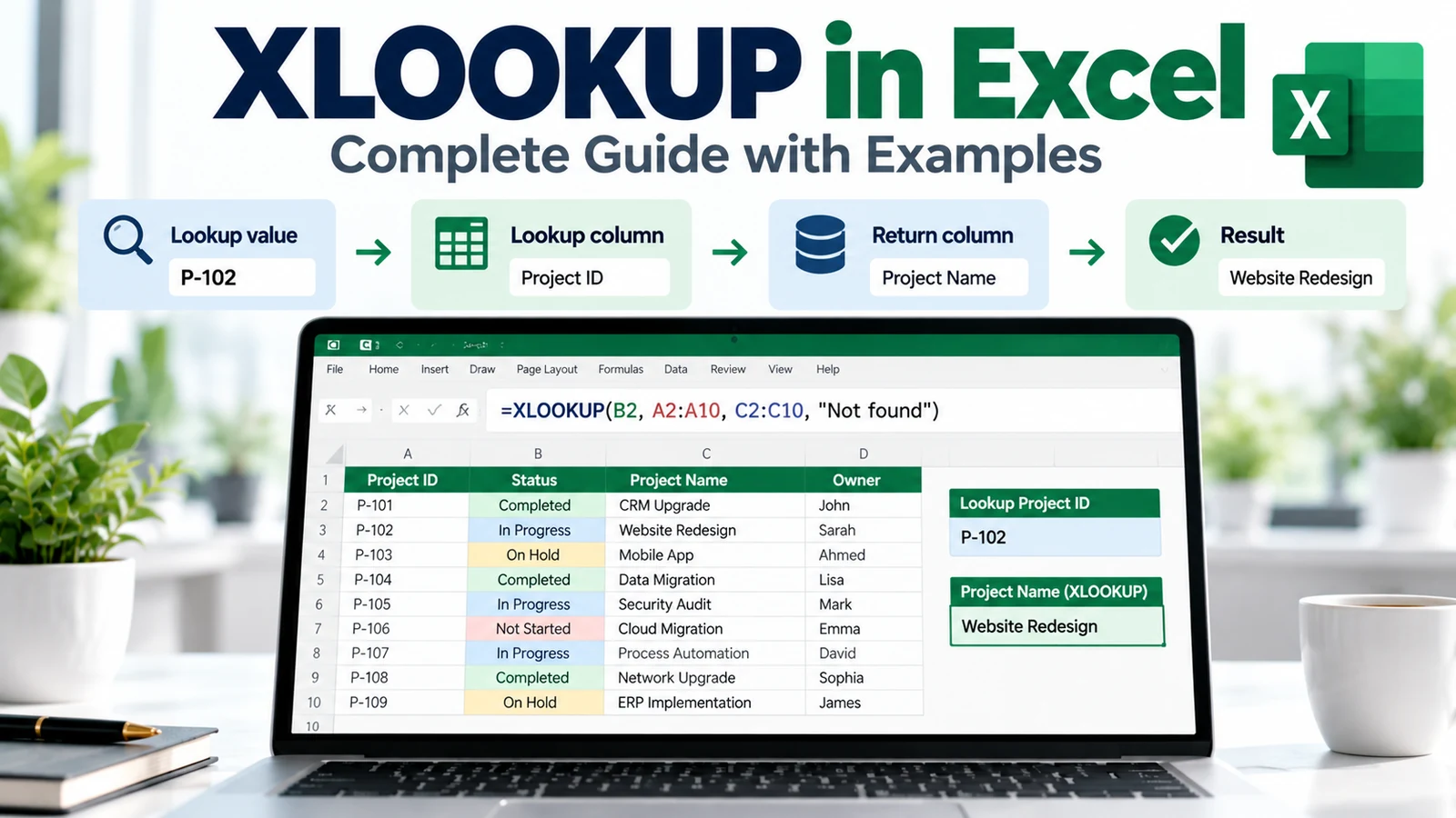
XLOOKUP in Excel is one of the most useful modern lookup functions for finding a value in one range and returning the corresponding value from another. It is easier to read than many older lookup formulas, supports exact matches by default, and can return values from columns located either to the left or the right of the lookup column.
This guide explains how to use XLOOKUP in Excel step by step, from the basic syntax to not-found handling, left lookups, multiple return columns, wildcard searches, approximate matches, nested XLOOKUP formulas, and practical project-management examples.
Microsoft describes XLOOKUP as a lookup and reference function that searches a range or array and returns the corresponding result from another range. Microsoft also recommends XLOOKUP as a more flexible alternative to VLOOKUP for modern Excel versions. See the official references for the XLOOKUP function, lookup and reference functions, and lookup alternatives in Excel.
If you are building your Excel skills progressively, start with the Microsoft Excel Learning Hub and the Excel Formulas & Functions guide. XLOOKUP becomes especially useful when you later combine formulas with Excel dashboards, PivotTables, or Power Query.
What Is XLOOKUP in Excel?
XLOOKUP searches for a value in one range and returns a corresponding value from another range.
For example, suppose a project list contains:
| Project ID | Project Name | Project Manager | Status |
|---|---|---|---|
| P-101 | Network Upgrade | Maria | On Track |
| P-102 | CRM Migration | David | At Risk |
| P-103 | Cloud Transition | Aisha | On Track |
If cell G2 contains P-102, you can return the project manager with:
=XLOOKUP(G2,A2:A4,C2:C4)The result is:
DavidXLOOKUP Syntax
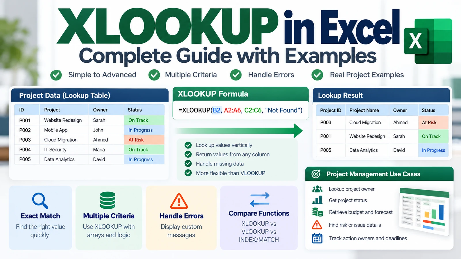
The standard syntax is:
=XLOOKUP(lookup_value, lookup_array, return_array, [if_not_found], [match_mode], [search_mode])| Argument | Purpose |
|---|---|
| lookup_value | The value you want to find. |
| lookup_array | The range Excel searches. |
| return_array | The range containing the value to return. |
| if_not_found | Optional value to return when no match exists. |
| match_mode | Optional control for exact, approximate, or wildcard matching. |
| search_mode | Optional control for search direction or binary search. |
Basic XLOOKUP Example
Suppose column A contains employee IDs and column B contains employee names:
A2:A100 → Employee ID
B2:B100 → Employee Name
If cell E2 contains an employee ID, use:
=XLOOKUP(E2,A2:A100,B2:B100)XLOOKUP searches column A and returns the matching name from column B.
XLOOKUP Uses Exact Match by Default
One of the biggest differences from VLOOKUP is that XLOOKUP uses exact matching by default.
You do not need to add FALSE just to request an exact match.
For example:
=XLOOKUP("P-102",A2:A100,D2:D100)This searches for the exact project ID P-102 and returns the corresponding value from column D.
Use XLOOKUP with a Cell Reference
In real workbooks, it is usually better to store the search value in a cell rather than hard-code it inside the formula.
For example:
=XLOOKUP(G2,A2:A100,D2:D100)This makes the formula reusable because users can change the value in G2 without editing the formula.
A drop-down list in Excel can make this even more user-friendly by letting users select the project, owner, region, or status from a controlled list.
Handle Missing Values with if_not_found
If XLOOKUP cannot find a match, Excel normally returns #N/A.
You can provide a cleaner message with the optional if_not_found argument:
=XLOOKUP(G2,A2:A100,D2:D100,"Not found")Now the formula returns:
Not foundinstead of an error.
XLOOKUP Can Look to the Left
Traditional VLOOKUP requires the lookup column to be on the left side of the return column.
XLOOKUP does not have that restriction.
Suppose:
B2:B100 → Project Name
A2:A100 → Project ID
You can search the project name and return the project ID:
=XLOOKUP(G2,B2:B100,A2:A100)This is often called a left lookup.
Return Multiple Columns with XLOOKUP
In modern Excel, XLOOKUP can return several adjacent columns at once.
For example:
=XLOOKUP(G2,A2:A100,B2:D100)If the return array covers columns B through D, Excel can spill the matching values across neighboring cells.
This is useful when one search should return:
- Project Name
- Project Manager
- Status
XLOOKUP with Excel Tables
Structured references make formulas easier to understand.
If your table is named ProjectData, you might use:
=XLOOKUP(G2,ProjectData[Project ID],ProjectData[Status],"Not found")This is easier to maintain than a formula using fixed cell ranges.
XLOOKUP Match Modes
The optional match_mode argument controls how XLOOKUP handles matching.
| match_mode | Meaning |
|---|---|
| 0 | Exact match — default |
| -1 | Exact match or next smaller item |
| 1 | Exact match or next larger item |
| 2 | Wildcard match |
Wildcard XLOOKUP
Wildcard matching can be useful when the lookup value is only part of the text.
Excel supports common wildcard characters:
*— any sequence of characters?— one character
Example:
=XLOOKUP("*Cloud*",B2:B100,D2:D100,"Not found",2)This searches for text containing the word Cloud.
Approximate Match with XLOOKUP
Approximate matching is useful for ranges such as thresholds, grades, discounts, or risk bands.
Suppose you have:
| Minimum Score | Rating |
|---|---|
| 0 | Low |
| 40 | Medium |
| 70 | High |
| 90 | Critical |
You can use:
=XLOOKUP(G2,A2:A5,B2:B5,"Not found",-1)The -1 match mode returns an exact match or the next smaller value.
XLOOKUP Search Modes
The optional search_mode argument controls how Excel searches the lookup array.
| search_mode | Meaning |
|---|---|
| 1 | Search first to last — default |
| -1 | Search last to first |
| 2 | Binary search ascending |
| -2 | Binary search descending |
Find the Last Match
Searching from last to first is useful when a value appears several times and you want the most recent or final matching entry.
=XLOOKUP(G2,A2:A100,D2:D100,"Not found",0,-1)XLOOKUP with Multiple Criteria
XLOOKUP does not have a dedicated multiple-criteria argument, but you can combine logical tests.
Suppose:
A2:A100 → Project
B2:B100 → Month
C2:C100 → Status
If G2 contains the project and H2 contains the month:
=XLOOKUP(1,(A2:A100=G2)*(B2:B100=H2),C2:C100,"Not found")The two logical tests create an array of 1s and 0s. XLOOKUP searches for the row where both conditions are true.
Nested XLOOKUP for Two-Way Lookups
You can nest XLOOKUP when you need to identify both a row and a column.
For example, imagine a project budget table with project names in rows and months in columns.
A two-way lookup can follow this pattern:
=XLOOKUP(ProjectName,ProjectRange,XLOOKUP(Month,MonthHeaders,DataRange))This can be useful for budget, forecast, or resource matrices.
XLOOKUP vs VLOOKUP
| Capability | XLOOKUP | VLOOKUP |
|---|---|---|
| Exact match by default | Yes | No |
| Look left | Yes | No |
| Separate lookup and return ranges | Yes | No |
| Built-in not-found result | Yes | No |
| Return multiple columns | Yes in modern Excel | Not directly |
| Search last to first | Yes | No |
Microsoft describes XLOOKUP as an improved alternative to VLOOKUP for newer Excel environments because it works in any direction and uses exact matching by default.
XLOOKUP vs INDEX and MATCH
Before XLOOKUP, a common flexible lookup pattern was:
=INDEX(ReturnRange,MATCH(LookupValue,LookupRange,0))XLOOKUP often provides the same result more clearly:
=XLOOKUP(LookupValue,LookupRange,ReturnRange)INDEX/MATCH remains useful in older workbooks and some advanced models, but XLOOKUP is usually easier to read when it is available.
Project Management Example 1: Find the Project Owner
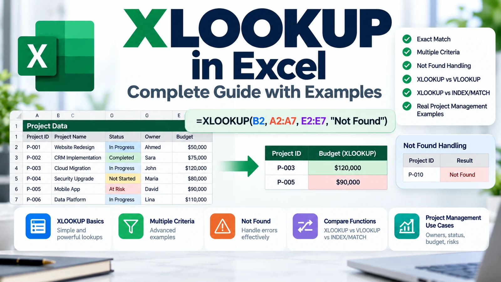
Suppose your project register includes:
Project ID | Project Name | Owner | Status | BudgetTo return the owner:
=XLOOKUP(H2,ProjectData[Project ID],ProjectData[Owner],"Project not found")This is useful for project trackers, governance sheets, and portfolio dashboards.
Project Management Example 2: Return Project Status
=XLOOKUP(H2,ProjectData[Project ID],ProjectData[Status],"Unknown")You can combine the result with conditional formatting to highlight values such as At Risk, Delayed, or On Track.
Project Management Example 3: Retrieve Budget Data
To return the approved budget:
=XLOOKUP(H2,ProjectData[Project ID],ProjectData[Approved Budget],0)You can then calculate variance using:
=ActualCost-ApprovedBudgetThese calculations can feed an Excel project dashboard containing KPI cards, budget variance charts, and slicers.
Project Management Example 4: Find a Risk Owner
Suppose a risk register contains:
Risk ID | Risk Description | Owner | Probability | Impact | StatusUse:
=XLOOKUP(H2,RiskData[Risk ID],RiskData[Owner],"Unassigned")This can support project reviews by quickly retrieving the accountable risk owner.
Project Management Example 5: Latest Status Entry
If a project appears several times in a status-history table, you can search from the bottom upward:
=XLOOKUP(H2,A2:A500,D2:D500,"Not found",0,-1)This returns the last matching status in the range.
XLOOKUP with Power Query and PivotTables
XLOOKUP is excellent for row-level retrieval, but it is not the right tool for every data problem.
Use:
- XLOOKUP when you need to retrieve a related value.
- Power Query when you repeatedly import, clean, merge, or transform data.
- PivotTables when you need aggregated summaries and flexible analysis.
- Excel dashboards when you need a visual reporting layer.
These tools work well together rather than replacing one another.
Common XLOOKUP Errors
#N/A
The lookup value was not found.
Use the optional not-found argument:
=XLOOKUP(G2,A2:A100,D2:D100,"Not found")#VALUE!
The lookup array and return array may not have compatible dimensions.
Unexpected Match
Check whether:
- Text contains leading or trailing spaces.
- Numbers are stored as text.
- The wrong match mode is being used.
- The wrong lookup column was selected.
Formula Not Available
Microsoft notes that XLOOKUP is not available in Excel 2016 or Excel 2019. If a workbook must support older desktop versions, consider INDEX/MATCH or VLOOKUP instead.
XLOOKUP Best Practices
- Use Excel Tables and structured references when possible.
- Keep lookup and return ranges the same size.
- Use meaningful not-found messages.
- Prefer cell references over hard-coded values.
- Use exact match unless approximate matching is intentional.
- Document advanced match and search modes.
- Keep lookup keys unique when the model expects one result.
- Use Power Query instead of complex lookup chains when the real task is repeated data merging.
Frequently Asked Questions About XLOOKUP in Excel
Is XLOOKUP better than VLOOKUP?
For many modern Excel use cases, XLOOKUP is easier to read and more flexible because it can look in either direction, uses exact match by default, and separates the lookup range from the return range.
Can XLOOKUP return multiple values?
Yes. In modern Excel, XLOOKUP can return multiple adjacent columns when the return array spans several columns.
Can XLOOKUP use multiple criteria?
Yes. You can combine logical tests into an array and search for the row where all criteria evaluate to true.
Can XLOOKUP replace INDEX/MATCH?
In many lookup scenarios, yes. INDEX/MATCH remains useful for compatibility and some advanced models, but XLOOKUP often expresses the same logic more simply.
Can XLOOKUP search from bottom to top?
Yes. Use -1 as the search mode to search from the last item to the first.
Does XLOOKUP work in Excel 2016 or Excel 2019?
No. Microsoft states that XLOOKUP is not available in Excel 2016 or Excel 2019, although those versions may display a workbook created in a newer version that contains the function.
Continue Learning
Final Takeaway
XLOOKUP in Excel simplifies one of the most common spreadsheet tasks: finding a value and returning related information from another range.
For most modern lookup scenarios, the core pattern is simple:
=XLOOKUP(WhatYouNeedToFind,WhereToSearch,WhatToReturn)Once you understand that pattern, you can extend it with not-found messages, wildcard matching, approximate matching, reverse searches, multiple criteria, and project-management use cases. Use XLOOKUP for targeted retrieval, Power Query for repeatable data preparation, PivotTables for aggregation, and dashboards for visual decision support.